“I need two GPUs.”
A user can describe the request in four words. The application still has several decisions to make: which job gets considered next, which resources it can receive, and how to keep track of that assignment until the resources are released.
I built my workload-management project to make those decisions visible. It models requests, allocations, and job states; workload execution belongs to a separate layer.
Prefer a visual journey? Follow the request through an interactive allocation story.
A place in the queue
Consider four eligible machines, or Nodes, arranged in one row of a mesh. Each has one GPU. A new job, Job 42, asks for any two GPU units. Its client and quota checks have passed. The IDs and resource states in this example are illustrative.
| Machine | Coordinates | GPU unit | At submission |
|---|---|---|---|
| Node 11 | (0, 0) | 71 | In use by another job |
| Node 12 | (1, 0) | 87 | Free |
| Node 13 | (2, 0) | 91 | Held by an earlier job |
| Node 14 | (3, 0) | 95 | Held by that same earlier job |
With only one GPU free, the request must wait. The queue can follow arrival order or job priority. By default, if the next job needs more capacity than is free, it stays queued and the application does not try the jobs behind it.
When the earlier job is marked complete, GPUs 91 and 95 are released and the queue is checked again. There are now three free GPU units for our two-GPU request. GPU 71 on Node 11 is still occupied.
Choosing the two GPUs
There is enough capacity now, but more than one way to satisfy the request.
The placer first checks whether one machine can supply both GPUs. Here, each machine has only one, so the assignment must span machines.
With Pack, free candidates nearer to existing occupied nodes are preferred. Node 11 provides that occupied reference: Nodes 12, 13, and 14 are one, two, and three coordinate steps away. Pack therefore selects GPU 87 on Node 12 and GPU 91 on Node 13.
With Spread, the preference is reversed. From the same inventory, it would select GPU 95 on Node 14 and GPU 91 on Node 13. Both choices satisfy the requested quantity; they express different placement preferences.
This is why I keep two questions separate. The Scheduler decides which queued job gets an attempt. The Placer decides which exact resource units it receives. Changing the placement preference leaves queue ordering independent.
The cluster defines the layout
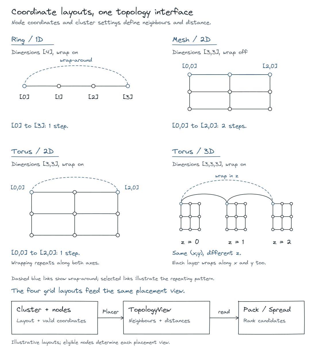
Those distances come from the cluster’s configuration. Each node’s coordinates are checked against the cluster’s dimensions. For each placement attempt, the placer builds a fresh TopologyView over the eligible nodes, including occupied nodes that provide spatial context.
Pack and Spread use that view’s distances to rank candidates. Keeping the geometry there lets the policies work across the supported grid layouts. A cluster’s dimensions and wrap-around setting determine what “nearby” means.
Inside the architecture: queue order, placement, and object lifetimes
The Server coordinates the attempt. The process-local queue retains job IDs and priority; the job and locked inventory are loaded for the current database session. SortStrategy and PlaceAlgorithm provide the two independent policy interfaces.
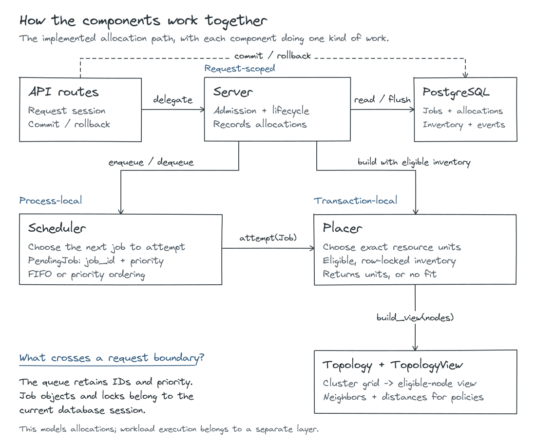
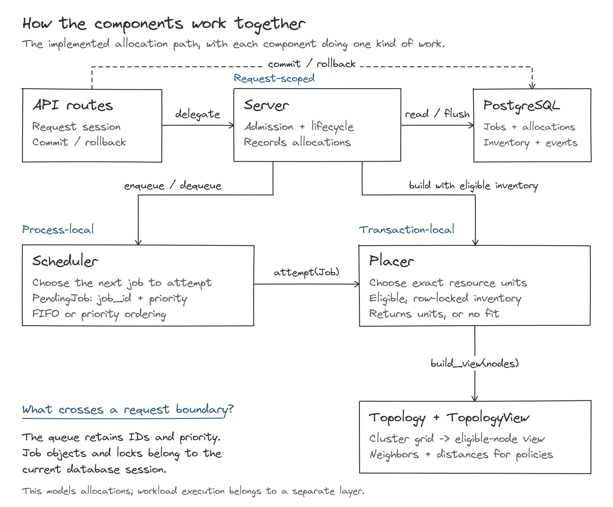
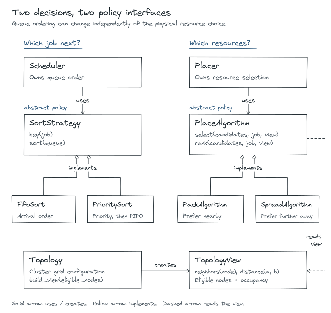
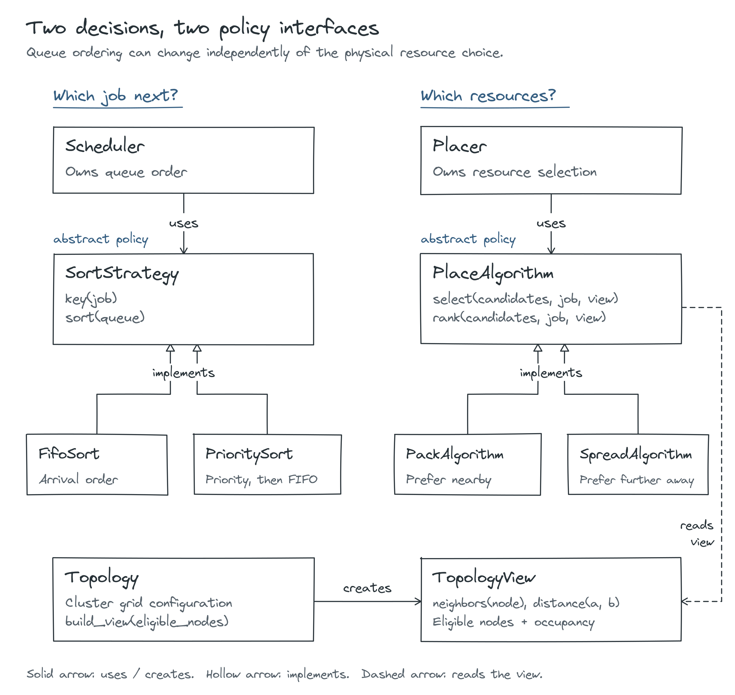
The project case study includes the complete class architecture and ERD. The Pack and Spread article examines the placement preferences in more detail.
See how ring, mesh, and torus layouts change coordinate distance
In our example, the mesh has a single row and does not wrap. These other configurations show how the same distance interface interprets different layouts.
A free GPU can still be unreachable
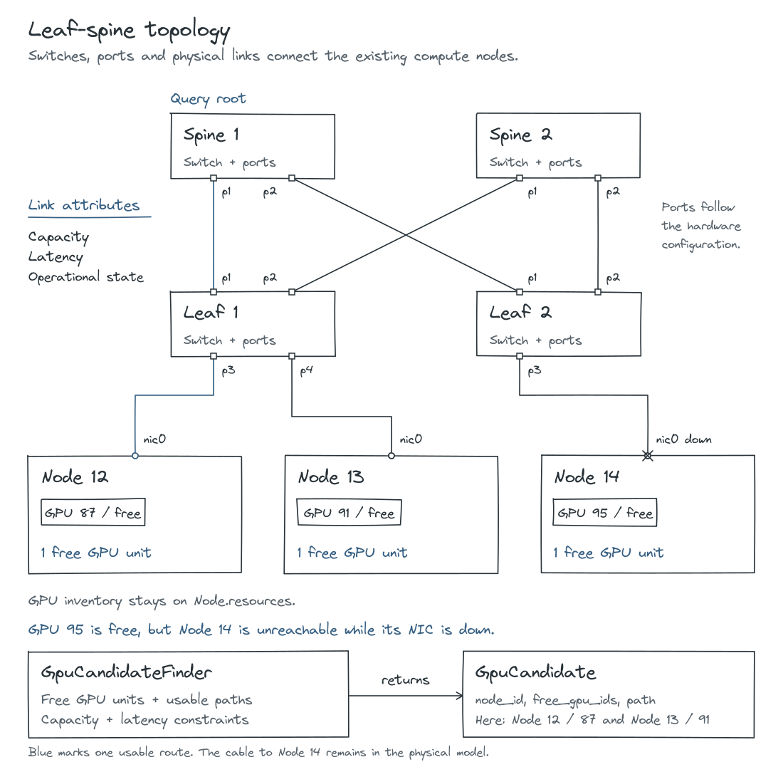
A machine’s GPU can be free while its NIC is down.
In the leaf–spine model, compute nodes attach to leaves, which connect through spines. GpuCandidateFinder combines the nodes’ existing GPU inventory with operational paths from a selected root switch. The query can apply configured capacity and latency limits and returns free GPU IDs together with paths.
Consider a fabric query on the three free nodes above. If Node 14’s NIC is down, GPU 95 remains free in the inventory but is excluded from the query result. A coordinate view describes distance; the fabric query establishes which candidates are reachable under its constraints.
Remembering the decision
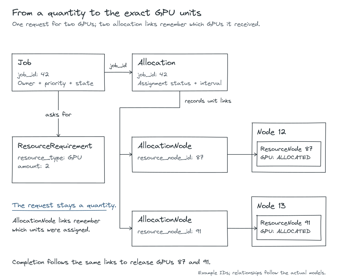
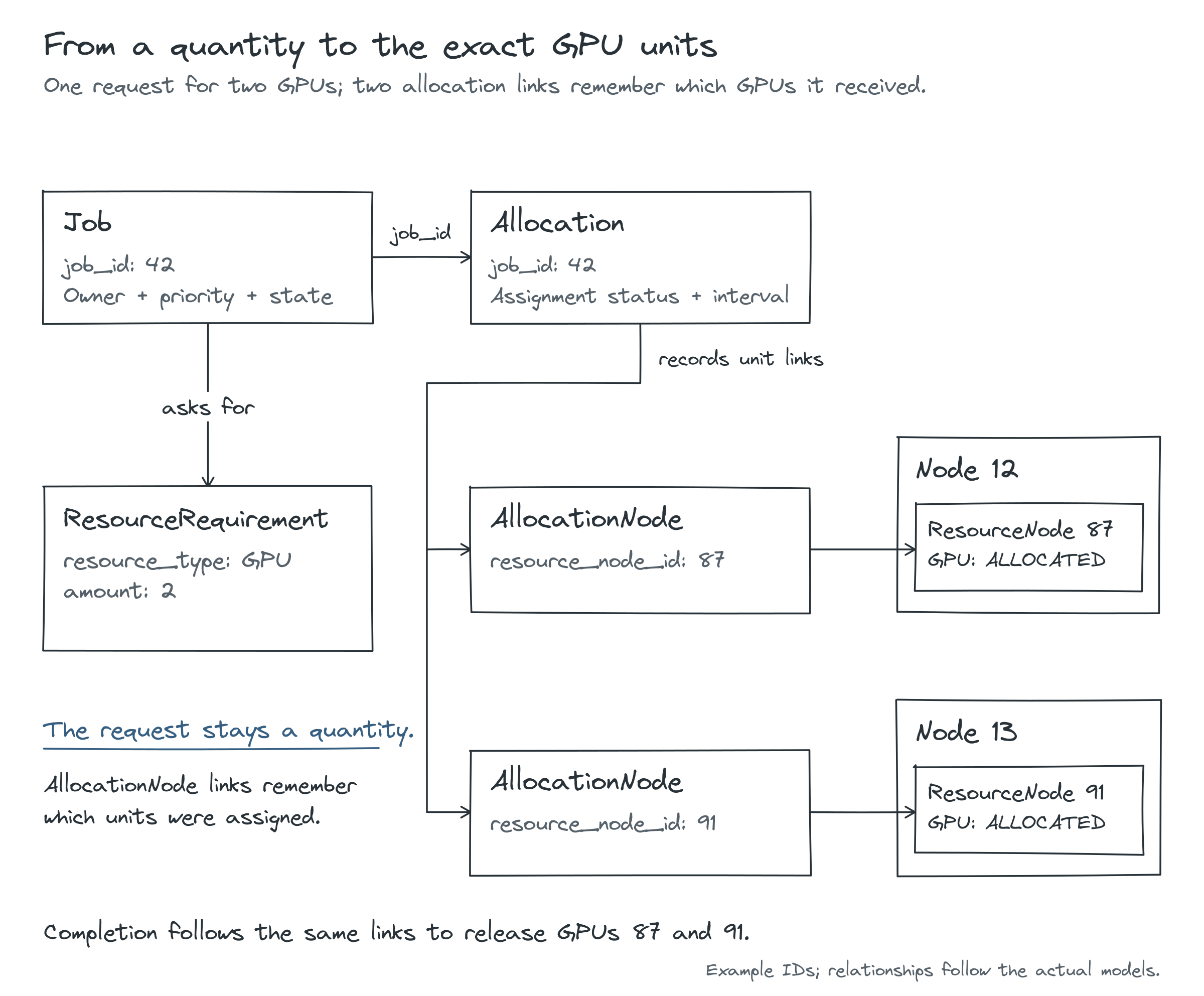
Job 42 now receives GPU 87 on Node 12 and GPU 91 on Node 13, following the Pack choice.
The original request still says “two GPUs.” The assignment must identify these exact units. I keep the request and its fulfillment as separate records: ResourceRequirement preserves the quantity, while Allocation and its AllocationNode links record what the job received.
That gives the interface something concrete to display and tells the application what to release later. The resource-state changes, allocation records, and job-state update are committed together. In this model, the job then appears as running: resources have been assigned to it.
Giving the resources back
When Job 42 finishes or is cancelled, the application follows those allocation links and releases GPUs 87 and 91. It records the job’s history and checks the queue again.
But suppose Node 13 was taken out of service while the job held GPU 91. Releasing the assignment must preserve that decision. GPU 87 can become available on Node 12; GPU 91 must remain unavailable on Node 13.
The job’s claim on both GPUs has ended. Whether each GPU can be used again still depends on the machine’s state.